Sound consists of longitudinal waves: the particles of the medium through which a sound travels oscillate along the direction in which the sound is travelling. In air, this causes small compressions and rarefactions of pressure, above and below nominal atmospheric pressure. The corresponding movement of particles occurs one quarter of a cycle (90°) later.
The velocity of sound (c) varies slightly with temperature. At zero degrees celsius (0 °C) it’s about 331 metres per second (m/s), increasing by 0.54 m/s for every °C rise in temperature. Hence, at a typical room temperature of 18 °C, it’s approximately 340 m/s.
The frequency of a sound indicates the rate at which the sound waves are propagated, as measured in cycles per second. Nowadays, the term ‘cycles per second’ is replaced by a unit called the hertz (Hz), prefixed, as necessary, by k for multiples of 1,000. Hence 20,000 Hz is written as 20 kHz.
The wavelength of a sound is defined as the distance between corresponding points on successive sound waves. This is given by the equation:-
where
λ = wavelength in metres (m)
c = velocity of sound in
f = frequency in hertz (Hz)
The following table gives other useful figures:-
| Frequency (f) | Wavelength (λ) |
|---|---|
| 30 Hz | 11.3 m |
| 100 Hz | 3.4 m |
| 500 Hz | 680 millimetres (mm) |
| 1 kHz | 305 mm |
| 2 kHz | 170 mm |
| 10 kHz | 34 mm |
| 16 kHz | 21 mm |
The way in which the human ear responds to sound is defined by Weber’s Law, which states:-
‘Where any physiological stimulus varies by equal steps in a geometric progression, perception of the stimulus varies by equal steps in an arithmetic progression’.
If it helps, try comparing the geometric sequence of 2, 4, 8, 16 with the arithmetic progression of 1, 2, 3, 4. In essence, this law indicates that the ear responds to sound volume in a logarithmic manner, so that a tenfold increase in sound pressure is only felt as a doubling of intensity. Similarly, doubling the frequency of a sound is only perceived as a change of one octave.
The human ear responds to frequencies between 20 and 20,000 cycles per second, although children can often hear up to 30 kHz whilst older people have a more limited range. Fortunately for the latter, human speech is mainly confined to the region between 300 Hz and 3 kHz. An electronic music synthesiser, on the other hand, can produce frequencies as low as 5 Hz and beyond 20 kHz. Those frequencies above the human range of hearing are known as ultrasonic, and the sounds themselves as ultrasound. Although used in technology, such sounds are outside the scope of this article.
Most acoustic musical instruments produce harmonics at multiples of a fundamental frequency. If f is the fundamental then the even harmonics are:-
whilst the odd harmonics are:-
Note that the latter frequencies produce what is usually considered to be a less musical sound.
The range of frequencies produced by instruments and other sound sources are given below:-
| Source | Lowest (Hz) | Highest (kHz) |
|---|---|---|
| Violin | 180 | 16.0 |
| Viola | 140 | 16.0 |
| Cello | 70 | 10.7 |
| Bass Violin | 40 | 7.5 |
| Piccolo | 520 | 9.25 |
| Flute | 300 | 13.5 |
| Oboe | 300 | 16.0 |
| Clarinet | 155 | 9.5 |
| Bass Clarinet | 75 | 10 |
| Bassoon | 25 | 9.13 |
| Trumpet | 155 | 9.5 |
| French Horn | 110 | 6.2 |
| Trombone | 75 | 8.0 |
| Bass Tuba | 45 | 6.2 |
| Piano | < 30 | 6.2 |
| 32 or 64 ft | < 20 | - |
| Bat's Location | - | > 20 |
For convenience, the measured level of a sound should match its subjective volume. The value of any sound pressure level (SPL) can be expressed in decibels (dB) using the following equation:-
where P is the sound pressure and Po is a reference known as the threshold of hearing. This reference, corresponding to 0 dB, is equivalent to a pressure of 20 micropascals (µPa) or 0.002 dyne/cm2. The ear accepts a sound power of between 10 µW/m2 and 10 W/m2, a range of over 120 dB. The level of 130 dB is known as the threshold of pain or threshold of feeling.
The voltage gain or loss of an electrical circuit, as measured in dB, is given by the equation:-
where V1 and V2 are the voltage levels at the circuit’s input and output respectively. The following points are worth noting:-
If V1 > V2 then Av is positive
If V1 = V2 then Av = 0 dB
If V1 < V2 then Av is negative
We can measure an absolute signal level by making V2 equal to a reference voltage.
Where reference voltages other than 775 mV are used, the dB term usually carries a suffix. For example, dBm refers to a power reference of one milliwatt (1 mW) into a load impedance of 600 Ω (ohms), although in practice it often refers to the corresponding voltage of 775 mV. Other terms are also used, as shown below:-
| Term | Reference |
|---|---|
| dBr | 775 mV or other |
| dBu | 775 mV |
| dBv | 1 volt (V) |
Decibels are particularly useful for calculating gain and loss, since addition and subtraction are used instead of multiplication and division. For example, if we apply a signal of -40 dBr to a 20 dB amplifier the output is given by:
and if we apply a signal of -30 dBr to a 20 dB attenuator the output is:
The following table gives useful figures for gain and loss ratios:-
| dB | Gain | Loss |
|---|---|---|
| 0.1 | 1.01 | 0.989 |
| 0.5 | 1.06 | 0.944 |
| 1.0 | 1.12 | 0.891 |
| 1.5 | 1.19 | 0.841 |
| 2 | 1.26 | 0.794 |
| 3 | 1.41 | 0.708 |
| 4 | 1.58 | 0.631 |
| 5 | 1.78 | 0.562 |
| 6 | 1.99 | 0.501 |
| 7 | 2.24 | 0.447 |
| 8 | 2.51 | 0.398 |
| 9 | 2.82 | 0.355 |
| 10 | 3.16 | 0.316 |
| 12 | 3.98 | 0.251 |
| 14 | 5.01 | 0.199 |
| 16 | 6.31 | 0.158 |
| 18 | 7.94 | 0.126 |
| 20 | 10.00 | 0.100 |
| 30 | 31.60 | 0.032 |
| 40 | 100 | 0.010 |
| 50 | 316 | 0.003 |
| 60 | 1000 | 0.001 |
| 70 | 3160 | 0.0003 |
| 80 | 10000 | 0.0001 |
| 90 | 316000 | 0.00003 |
| 100 | 100000 | 0.00001 |
Intermediate values can also be calculated from such a table, such as:-
11 dB = (10 + 1) dB
∴ Gain Ratio
38 dB = (40 - 2) dB
∴ Gain Ratio
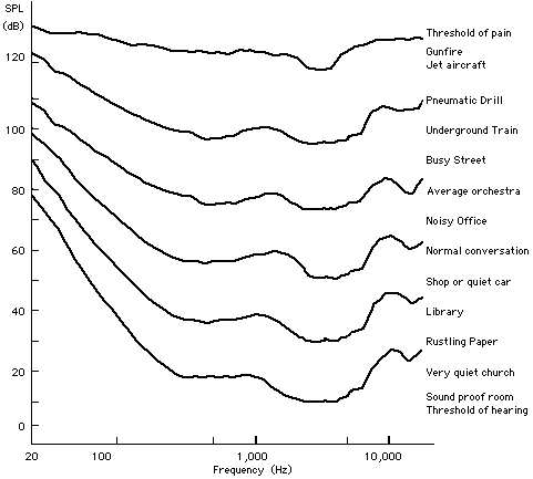
The sensitivity of the human ear, and hence the subjective loudness of a sound, varies with frequency. This is shown in Fletcher Munson’s equal loudness contours, illustrated below:-
The curving lines demonstrate the subjective loudness at different frequencies.
Several different weighting curves are used to modify SPL readings so as to make them more closely match the response of the human ear. They’re mainly of academic interest, but are included here for completeness. The most common ‘A’, ‘B’, ‘C’ and ‘D’ weightings are shown below:-
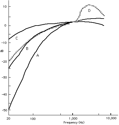
Unfortunately, none of these are ideal for all situations or every sound. The above weightings are described as follows:-
This curve, intended for measuring SPLs below 40 dB, is specified in IEC Standard 268. Signals should be measured using an RMS-reading meter, as defined in IEC Standard 651.
Now rarely used, although originally intended for SPLs between 40 and 70 dB.
Again rarely used, this ‘flat’ response is intended for SPLs over 70 dB.
Also rarely used, although intended for measuring aircraft noise and also known as the ‘N’ curve. It gives readings that are about 13 dB higher than the ‘A’ curve
Other common weighting characteristics include:-
Similar to the older DIN (German Industry Standard) 45 405, requiring a special quasi-peak reading meter. This is often used for measurements of noise in electronic audio equipment.
This method was introduced by Dolby Laboratories and is similar to the above, but employs an average-reading meter and a 0 dB reference frequency of 2 kHz instead of 1 kHz.
The minimum amount of background noise produced by an electronic circuit is given by:-
where
V = noise voltage
k = Boltzmann’s constant
T = absolute temperature
R = circuit resistance
B = bandwidth in hertz (Hz)
Although equipment can be designed for the least possible noise, nothing can reduce it below this minimum, which is set by the laws of physics. For 200 or 600 Ω sources, the minimum noise voltage corresponds to -130 and -125 dBm respectively.
The signal-to-noise ratio (S/N) of a real electronic device, measured in dB, is obtained by comparing the peak level of noise with the peak level employed for actual ‘programme’ material. For example, a device that produces noise at -70 dBm and handles signals up to a maximum of +8 dBm has a S/N figure of 78 dB. However, such an S/N value doesn’t account for the sensitivity of the human ear at different frequencies, requiring the application of a weighting characteristic, such as one of the CCIR standards described above. This results in what appears to be an ‘improved’ noise figure.
©Ray White 2004.
